Buoyant Economies
Impact of the Floating Exchange Rate System on Employment and Growth
![]()
The floating exchange rate system
- Real gross domestic income grew at an annual rate of 4.2% per annum in the USA between 1949 and 1973. From when the US exchange rate was floated in March 1973, the rate of economic growth has declined to average 2.7% up until 2011. In Australia, real gross domestic income was growing at an annual rate of 5.2% per annum between 1960 and 1973. That was under the fixed exchange rate system. Between 1973 and 1983, after the USA had floated its currency but before Australia had floated, the average real rate of economic growth in Australia declined to 2.0%. Since 1983, when Australia floated its exchange rate, real gross domestic income has grown at an average rate of 3.8% per annum (to 2009). Rather than raising the rate of economic growth, floating the exchange rate has slowed the rate of economic growth by 34% in the USA and 27% in Australia.
Wages
- Floating the dollar has had an effect on wages growth. In the USA, average weekly earnings for the private non-farm sector was rising at 1.2% per annum in real terms, from 1964 to 1972, immediately before the US dollar was floated. In the next 20 years they declined at an average rate of 1.2% per annum. Then, between 1992 and 2004, they have been rising slowly at an average rate of 0.6% per annum in real terms: half the rate of the first period. Even so, average real wages for private non-farm workers in the USA in 2010 are still 16% below the levels they were in 1972 as shown in Figure 1. If average real wages in the US had maintained their pre-float growth rate, they would be 70% higher than they are today.
Figure 1. USA: Average Weekly Wages at constant 1992 prices for all private non-farm workers
Source: US Bureau of Labour Statistics
- In Australia, average real wages were rising up until June 1984. The real rate of wages growth had been around 4% between 1969 to 1975. Then it slowed to 0.6% until 1983 when Australia floated its dollar. It jumped more than 8% in the year to June 1984 following the float, when the value of the Australian dollar declined rapidly. In the six years from June 1984 to June 1990, average real wages declined at an average rate of more than 1.6% per annum. Since then, average real wages have been rising at about 1.4% per annum. Despite this improvement, the rate of real wages growth is less than half the rate it was in the 1960’s and 70’s. Average real wages did not return to their June 1984 levels again until June 2003. That is, Australia experienced nineteen years without any growth in average real wages above 1984 levels. Average real weekly wages for Australian workers are shown in the Figure 2. As minimum wages are regulated in Australia, Australian workers did not experience the same dramatic reduction in wages as in the USA.
Figure 2. Australia: Average Real Weekly Wages (Discounted by CPI base 1989/90)
Unemployment
- Floating the dollar also affected unemployment. In the USA, the rate of unemployment has increased significantly since 1973 when the US dollar was floated, as shown below in Figure 3.
Figure 3. USA: Unemployment Rate
Figure 4. Australia Unemployment Rate
Source: R.G. Gregory “A Longer Run Perspective on Australian Unemployment" & Australian Bureau of Statistics
In 1973, when the US dollar was floated, the Australian dollar was tied to the US dollar. From September 1974, the Australian dollar was tied to a basket of currencies until it was floated in December 1983. These links to other floated currencies help explain why Australia was affected by the floating exchange rate system, even before it had adopted the system.
Attaining equilibrium under fixed exchange rates
-
The main reason for the decline in wages growth and the rise in the level of unemployment is due to the way the fixed and the floating exchange rate systems attain equilibrium between foreign receipts and foreign payments.
Unemployment
-
The following charts explain the issue. The output, income, imports and exports of an economy are represented on the horizontal axis. The real exchange rate (on the vertical axis) is fixed at e1. In Figure 5, the economy is initially at equilibrium with exports (the supply of which is represented by the X1-X1 line) equal to imports (the demand for which is represented by the M1-M1 line) at the point A1. The total national income or output of the economy is at the point Z1. The economy earns income from two sources:
exports equal to 0-A1; and
domestic sales of A1-Z1.
It spends 0-A1 on imports and A1-Z1 on domestic products (which generates the domestic sales).
Figure 5. The initial equilibrium position (fixed exchange rate)
-
In Figure 6, we assume that there is a permanent increase in the supply of exports from the X1-X1 line to the X2-X2 line. As the exchange rate is fixed, exporters will supply exports of 0-A2. The income from exports will be equal to 0-A2 while the income from domestic sales will initially be at A1-Z1. Adding the income from exports to the income from domestic sales raises total income to 0-Z2 There is now disequilibrium in the economy with the foreign revenue from exports exceeding foreign payments on imports. Also, national income, or output, exceeds national expenditure.
-
The increased national income enables the economy to increase its spending. This expenditure is directed at both domestic products and imports. The proportion of spending spending on domestic products and imports will tend to be fixed because the relative prices of imports are fixed (because the exchange rate is fixed). The proportion of additional income spent on imports is called the 'marginal propensity to import'. The expenditure on domestic products raises the income of those that produced and sold the products. Therefore, it further raises national income. The expenditure on imports does not raise national income. National income will continue to rise while the income form exports is greater than spending on imports. When export income is equal to import payments, the economy will stop growing and return to equilibrium.
Figure 6. Disequilibrium- an increase in exports (fixed exchange rates)
-
This growth in income from export sales is known as the multiplier effect. The value of the export multiplier is equal to the inverse of the marginal propensity to import. Thus if a country spends 10% of its additional income on imports, a $1 billion increase in exports would increase national income by $10 billion. That is, when the national income has increased by $10 billion, the economy would be spending 10% of that, $1 billion, on additional imports. At that point the additional spending on imports would be equal to the additional income from exports and the economy would be at equilibrium again.
-
This new equilibrium position is shown in Figure 7. National income has increased to 0-Z3 with exports equal to 0-A2 and the income from domestic sales equal to A2-Z3. With the higher level of income, expenditure on, or demand for, imports would have shifted to line M2-M2 with spending on imports increasing to 0-A2. The mechanism for achieving equilibrium in an environment of fixed exchange rates is to raise or lower demand for imports by raising (or lowering) aggregate demand (and thereby national income).
-
It was in such an environment of fixed exchange rates that growth in export income was able to stimulate the economies of countries such as Australia and the US so that they experienced wages growth and high level of employment. This was possible despite strong union pressure to raise wages. Demand for labour was high and there was full employment.
Figure 7. New equilibrium- imports rise to equal exports (fixed exchange rates)
Attaining equilibrium under floating exchange rates
-
The effect of floating the dollar
is described below. Figure 8
presents a similar equilibrium position to that considered in Figure 4.
Exports and imports are equal at 0-A1 with income from
and spending on domestic products equal to A1-Z1.
The exchange rate is floating and is assumed to be initially at e1.
Figure 8. Initial equilibrium with floating exchange rates
-
As in Figure 6 for fixed exchange rate system above, in Figure 9 we now assume that there is a permanent increase in the supply of exports from the X1-X1 line to the X2-X2 line. As the exchange rate is now variable and set in the market to ensure that international payments and receipts are equal (at equilibrium), the exchange rate rises from e1 to e2. At the new exchange rate, spending on imports rise from 0-A1 to 0-A2 to equal exports. Imports increase because the higher exchange rate makes them cheaper. In the same way as for the example with fixed exchange rates, the income from exports has increased form 0-A1 to 0-A2. However, the higher exchange rate has made domestic products relatively more expensive and so spending on domestic products declines from A1-Z1 to A2-Z1 following the increase in spending on imports rising from 0-A1 to 0-A2. Therefore, despite the increase in exports, national income and aggregate demand has remained constant at Z1. Export growth no longer stimulates the whole economy.
Figure 9. New equilibrium with increased exports (floating exchange rates)
-
Under floating exchange rates, the foreign exchange market changes the relative price of imports and domestic products to shift demand between domestic products and imports. International transactions no longer raise national income in the domestic economy. There is no need for national income and aggregate demand to change because the exchange rate moves (or floats) to continuously achieve equilibrium.
-
The change from fixed to floating exchange rates changed the means by which the economy achieve equilibrium. This slowed the rate of economic growth, increased unemployment and stopped wages growth in countries such as the US and Australia that shifted from fixed to floating exchange rates. Under the fixed exchange rate system, they had enjoyed high rates of economic growth, high levels of employment and wages growth, all generated by increased exports. Floating the exchange rate removed the forces of disequilibrium that had previously generated growth and prosperity.
Globalization
-
In the environment of floating exchange rates, the growth in exports increases imports and reduces local spending on domestic products. In such an environment, export and import industries grow more rapidly, relative to import competing industries that supply the domestic market. This growth in the relative size of exports and imports compared to the remainder of the economy has become known as globalization. In Australia, imports and exports increased from between 12% and 14% of national income to more than 20%. The Australian Government recognizes that the high exchange rate is a problem for domestic industries. In the Treasurer's 2011 budget speech he states that "the dollar is around post‑float highs and this makes it difficult for some sectors, particularly those that compete in international markets."
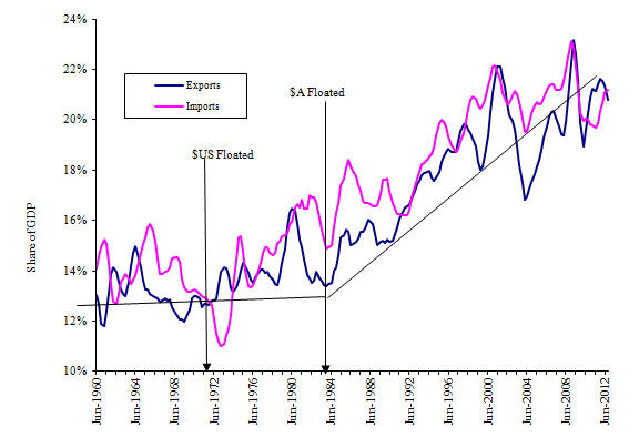
Figure 10. Australia: Exports and imports as a share of GDP
-
In the USA, exports and imports increased from between 4% and 5% of GDP to between 12% and 18% of GDP as shown in Figure 11.
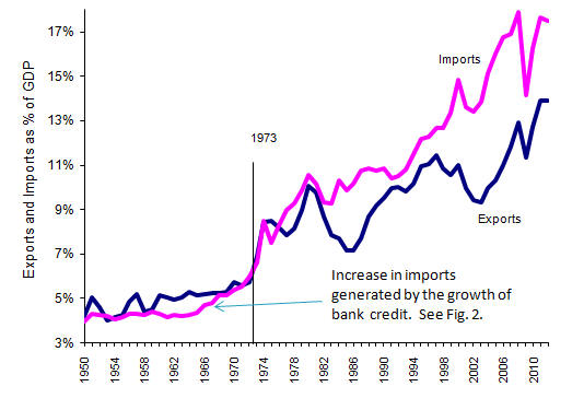
Figure 11. USA: Exports and imports as a share of GDP
-
This rise in the significance of imports and exports is represented in Figure 9 as the shift in exports and imports from 0-A1 (4%-5%) to 0-A2 (12%-18%).
-
While floating the dollar has increased trade as a share of GDP, trade would have been significantly higher if there had been fixed exchange rates. Figure 12 is uses to compare the effect of an increase in exports under the fixed exchange rate system and the floating exchange rate system.
-
Under the floating exchange rate system, an increase in the supply of exports from X1-X1 to X2-X2 would have prompted an increase in the exchange rate from e1 to e2 and an increase in exports and imports from A1 to A2. National income would have remained constant at Z1. Under the fixed exchange rate system, an increase in the supply of exports from X1-X1 to X2-X2 would have prompted an increase in exports from A1 to A3 and national income from Z1 to Z2. The amount of international trade associated with the floating exchange rate and globalisation is at A2 and is actually lower than the outcome with fixed exchange rates which would have reached equilibrium at A3. This lower level of trade was particularly hard felt in the ship-building industries in the mid to late 1970’s when countries such as the USA, UK and Germany floated their currencies. For example, evidence for this reduction in trade is evident in events such as the UK Shipbuilding (Redundancy Payments) Bill 1978.
Figure 12. Equilibrium with increased exports (comparing floating and fixed exchange rates)
-
The initial reduction in the growth of economic demand associated with the change from fixed to floating exchange rate was called the World Oil Crisis. This "spin", shifting the blame to OPEC, was accepted because the recession coincided with the OPEC decision to raise prices. However, while oil prices were high, they were not responsible for the recession. The recession had started before OPEC raised oil prices. Also, world trade did not recover when oil prices fell. Oil prices have fallen, risen and fallen again without the same significant changes in the world economy.
-
The US was able to eventually move out of recession by deregulating the growth of bank credit. However, bank credit has not been as effective at stimulating the economy as money from the growth of foreign reserves. Also, it has been more inflationary and caused current account deficits which have generally added to foreign debt. So far this century, the USA current account deficit has averaged $1.6 billion per day.
-
Since 1973, US exports have tripled relative to GDP. If US exports had tripled under a fixed exchange rate system US national income would have tripled, also. The floating exchange rate system has quarantined the US economy from receiving the benefits of trade growth and free trade. In addition, it has contributed to the rising level of foreign debt.
-
Australian exports have nearly doubled since 1983 despite the floating exchange rate system. If Australia had continued with fixed exchange rates, its national income would have been substantially higher, also. Floating the exchange rate has slowed economic growth, reduced real wages and raised foreign debt.
-
The floating exchange rate system has reduced world trade. Consequently, the whole world has been made poorer by it. Although China has continued to hold to its fixed exchange rate system, trade with China could have been greater if its trading partners had not adopted the floating exchange rate system.
-
The fixed exchange rate system generated economic growth, despite the inefficient labour market, without a major education campaign and without micro-economic reform. The floating exchange rate system has not been able to generate significant economic growth despite improvements in labour market efficiency, extensive investment in education, micro-economic reform and free trade agreements.
-
The reason for this is that these policies are attempts to shift the economy away from the stable equilibrium position. Efforts to improve productivity and make domestic products more competitive on both domestic and international market are attempts to move from equilibrium and force imports to fall and exports to rise. The floating exchange rate responds to such attempts to change relative prices by raising the exchange rate to make imports cheaper again. Therefore, no matter how a country tries to make its products more attractive, the exchange rate system will respond to restore the relative prices that bring equilibrium to the economy.
-
We do not need to return to fixed exchange rates to stimulate our economies. Market determined exchange rates can allow export to grow and raise aggregate demand to provide full employment. Trade driven economic growth can be achieved with external stability using a variable exchange rate system such as the guided exchange rate and liquidity system or the optimum exchange rate system. The principle behind the optimum exchange rate system is to provide incentives to the market to set the exchange rate at a level that would achieve full employment without excessive inflation. The economy is allowed to export more than it imports and thereby raise aggregate demand to a level that provides full employment. A model comparing the operation of the floating and optimum exchange rates systems is available here.
-
The principle of the optimum exchange rate system is explained in Figure 13 below. Assume that a country has income of Z1 with exports and imports equal to 0 - A1 and exchange rate e1. Full employment would be achieved if income were at Z2. Under the optimum exchange rate system, incentives are given to the financial system so that it maximise profits when there is full employment. Those incentives would encourage the financial market to drive the exchange rate towards e2. Exports would now exceed imports and so national income would rise. Exports would stop rising when imports have shifted the imports schedule from M1-M1 to M2-M2 so that imports equal exports at A2 and national income has increased to Z2 with sufficient income to raise demand to the level that provides full employment.
Figure 13. Achieving full employment with the Optimum Exchange Rate System
-
In this example, the export schedule stayed constant. It was the lower exchange rate that raised the proceeds of existing exports and stimulated additional exports so that export incomes rose to A2. It is the rise in income raises the demand for imports, shown as the shift in the import schedule. It is movement along the export schedule that causes national income rises to attain full employment. There is another model of the optimum exchange rate system in Figure 14 of the formula for the current account balance page. The optimum exchange rate system would raise incomes and allows policies designed to improve social welfare and the environment to be undertaken without causing harm to the economy or to employment levels.
-
Figure 14 below shows exports and imports in the Philippines as a share of gross national product. The Central Bank of the Philippines has modified its exchange rate system to maintain its international competitiveness. it has reduced the share of GNP that was spent on imports by nearly half, from 59 per cent in 1997 to 32 per cent in 2013. However, as in Figure 13, the economy has grown so much as a consequence of the rise in income that the real amount of imports have increased 61 per cent over that period, despite the reduced share of income spent on imports.
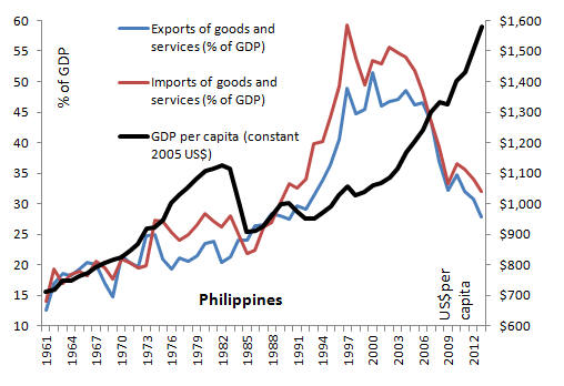
Figure 14. Philippines- exports and imports as a share of GNP (World Bank data)
-
While the approach in the Philippines is an ad-hoc approach it shows that the exchange rate system can be be used to increase national income and employment.
"I am the most unhappy man. I have unwittingly ruined my country. A great industrial nation is now controlled by its system of credit. We are no longer a government by free opinion, no longer a government by conviction and the vote of the majority, but a government by the opinion and duress of a small group of dominant men." Woodrow Wilson
Home
The impact of the floating exchange rate system on debt
Stimulating the UK economy while providing monetary and financial stability
Icelandic Economics - Olafur Margeirsson and the effect of floating
the exchange rate on Iceland
The effect of Money on Inflation
Formula
for the Current Account Balance
USA Australia New Zealand Philippines
Last update: 9 June 2016
Originally posted:1 November 2009